


In Parts 1 and 2, we have looked at the definitions of correlation, population and sample size. In this part, we will go through the essentials of the mathematics involved. Before we can proceed any further, however, we have to define certain fundamental statistical concepts.
Statistical Measures of a Data Set
In this section, it will be assumed that a data set is a sample drawn from some bigger population (for a definition of these terms, refer to my articles in Parts 1 and 2). There are a number of items that can be estimated about a data set. As an example, consider the data set consisting of 5 numbers that we used in Part 2:
X = [6 7 8 4 5]
Here, the symbol X is used to denote this entire set of numbers. An individual number in this data set is referred to by using subscripts on the symbol X to indicate a particular number, e.g. X2 refers to the 2nd number in X, namely the number 7; X4 refers to the 4th number in X, namely the number 4, and so on. Also, the symbol n will be used to represent the total number of elements in the set X. In our example, since our dataset consists of 5 numbers, n=5.
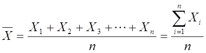
Mean: The mean is merely the arithmetical average of all the members of the data set. This value is obtained by adding together all the elements in the data set, and dividing the resulting sum by the total number of elements. Therefore, in our current example, if we add up all the five numbers in the data set X, a total of (6+7+8+4+5)=30 is obtained. Dividing this sum by the total number of elements in the data set, in this case 5, we get the mean of the data set: 30/5=6. Therefore the mean of the data set X is 6. The mean of the data set X is indicated by the symbol ![]() .
.
![]()
Writing out ![]() in this way can be unwieldy for bigger sets, i.e. larger values of n. Let me illustrate this with a simple example, for instance:
in this way can be unwieldy for bigger sets, i.e. larger values of n. Let me illustrate this with a simple example, for instance:
In the example above, the sum of all the numbers in dataset X can be expressed as:
X1 + X2 + X3 + X4 + X5
This is easy to do when the series of numbers to be added is small (n=5 in our example). But what if n were 100, or even a million? In that case, wouldn’t it be better to have a shorthand notation that can describe the summation in a compact and well-organized manner? Enter the Sigma Notation, derived from the Greek alphabet Σ. It is now possible to write the above summation as
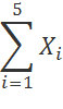
This notation just states the following: plug in 1 for the i in Xi, then plug 2 into the i in Xi, then 3, and so on all the way up to 5. Then, you add up the results. So that is X1 plus X2 plus X3, and so on, up to X5. Now tell me, would you still prefer to write out the sum the long, clumsy way, or would you rather use this much more elegant notation? If you want to do some further reading on the Sigma Notation, I would recommend this website. The Sigma Notation is only a handy technique that describes how to add up long series of numbers.
Using the Sigma Notation, the mean can now be denoted mathematically by the formula:
Unfortunately, the mean does not reveal much about the data except that it defines some kind of a midpoint (in technical jargon, this is known as a measure of central tendency). As an example, let us look at two other data sets Y=[6 6 6 6 6] and Z=[9 1 0 12 8], as shown in Table 1, and represented graphically in Figure 1. All these three data sets X, Y and Z have exactly the same mean (![]() 6), but are noticeably rather dissimilar. So what is it that is different about these three sets? The difference lies in the spread of the data (technically, this is called a measure of dispersion).
6), but are noticeably rather dissimilar. So what is it that is different about these three sets? The difference lies in the spread of the data (technically, this is called a measure of dispersion).
|
|
X |
Y |
Z |
|
1 |
6 |
6 |
9 |
|
2 |
7 |
6 |
1 |
|
3 |
8 |
6 |
0 |
|
4 |
4 |
6 |
12 |
|
5 |
5 |
6 |
8 |
|
Mean |
6 |
6 |
6 |
Table 1: Three datasets X, Y and Z
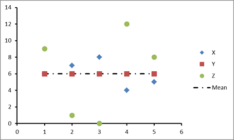
Figure 1: Datasets X, Y and Z shown graphically as values along the vertical axis
There are many ways of measuring the spread of a data set. In general, all of these describe the degree to which the data are dispersed around the mean value.
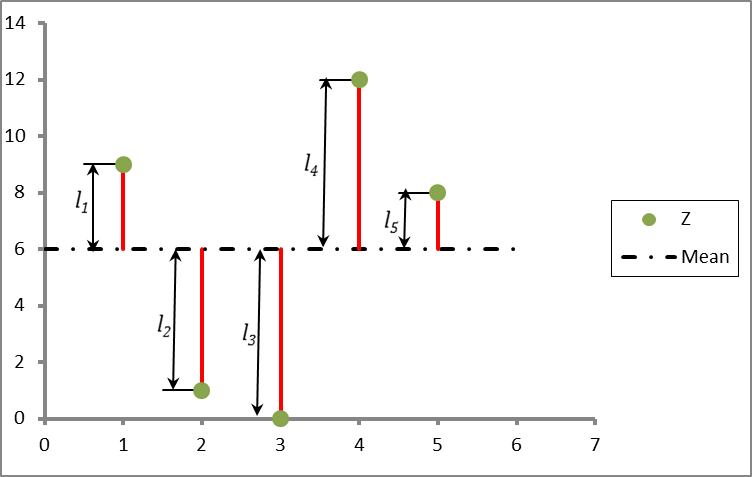
Figure 2: Dataset Z used as an example to show how the Squared Deviation is calculated
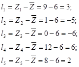
To illustrate the concept, let us use the data set Z to demonstrate how the deviations about the mean value are calculated. Figure 2 shows the elements of the data set Z graphically, as well as the mean value (which is ![]() as described above). The distances l1, l2,…, l5 represent how far each point Z1, Z2,…, Z5 lies from the mean line respectively. In other words, the deviation from the mean is the value obtained by subtracting the mean value from each element of the data set. It is very easy to calculate these distances. Thus, in mathematical terms:
as described above). The distances l1, l2,…, l5 represent how far each point Z1, Z2,…, Z5 lies from the mean line respectively. In other words, the deviation from the mean is the value obtained by subtracting the mean value from each element of the data set. It is very easy to calculate these distances. Thus, in mathematical terms:
Note the existence of both positive and negative values in the calculations above. But how can these deviation values be represented in a meaningful way? We could combine these values to form a single number, for example. If we followed a similar procedure to that performed for the calculation of the mean, we would add up all the values of the deviations l1, l2, …, l5 and divide the resulting sum by the total number of elements n = 5. Let us see what happens when we do this:
(l1+l2+l3+l4+l5)/n = (3-5-6+6+2)/5 = 0/5 =0,
not a very useful result! In fact, this is only to be expected: because the mean represents the average of the data set, the deviations above the mean are similar to those below it.
One clever way of getting around this problem is to square the deviations, thus making all the values positive. Using the same data set Z, we get:
l12 = 32 = 9;
l22 = (-5)2 = 25;
l32 = (-6)2 = 36;
l42 = 62 = 36;
l52 = 22 = 4
Let us see what happens when we add these values up, using the Sigma Notation described above:
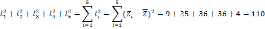
This is encouraging! Thus, the total squared deviation from the mean is 110.
As another example, the data set Y also has a mean value of 6, but its total squared deviation from the mean is zero, since all the elements have the same value of 6. None of the values deviate from the mean (l1 = l2 = … = l5 = 0). We can now calculate the mean or average of the squared deviation. Which leads us to the next definition….
Average Squared Deviation:
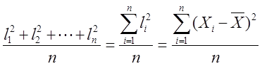
The average of the squared deviations from the mean is just the total squared deviation divided by the number of elements. We have calculated the total squared deviation in the above example to have the value 110. If we divide this by n, the total number of elements in the data set, we get the average of the squared deviations from the mean. In this example, the value is 110/5 = 22. In mathematical terms, the average squared deviation of a dataset X can be written as
Although the average squared deviation of a data set is a frequently used statistical measure of dispersion, it is only one of a list of measures that describes the degree to which the data are spread out around the mean value.
We will see later that the average squared deviation is connected to another statistical measure, known as the standard deviation. Before we get into a formal definition, however, it is useful to define another closely related measure: the variance.
Variance: The variance can also be regarded as another measure of the spread of data in a data set. The difference between the average squared deviation from the mean and the variance is that in the case of the latter, the sum of squared deviations from the mean is divided by the total number of items in the data set, n, minus one. Therefore, the variance for the data set Z is 110/(5-1) = 110/4 = 27.5.
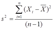
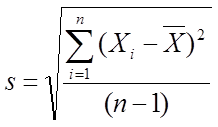
Following the formula for the average squared deviation above, and replacing the denominator by (n-1), the variance s2 can be written mathematically as:
A simplified tabular form of the calculations involved above for the average squared deviation and the variance, using data set Z as an example, is displayed below:
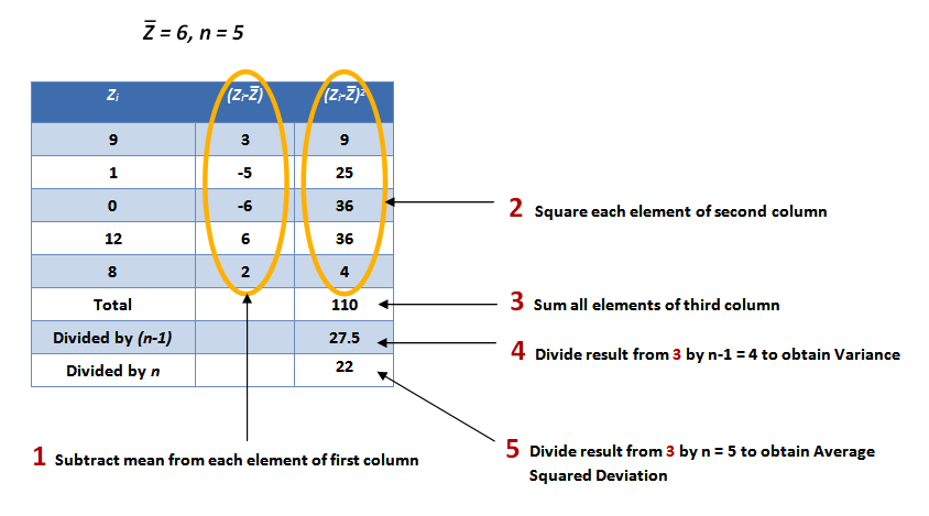
Table 2: Calculation of the average squared deviation and variance
The question immediately arises as to the usage of (n-1) instead of n. In general, a hand-waving answer is as follows: if the data set being used is a sample data set, i.e. it is a subset of the real-world (like choosing 500 US citizens randomly about their opinion regarding a particular celebrity figure), then one must use (n-1), because it is expected that the variation about the mean would be greater if the population mean were used. To compensate for this, the sum of squared deviations is divided by a slightly smaller number (n-1). It turns out that this simple tweak provides an answer that is closer to the variance which would have resulted from using the entire population, than if the value n were used in the denominator. As the sample size increases, the sample mean gets closer to the population mean, and the difference between the quotients based on n or (n-1) gets narrower. If, however, the calculation is not for a sample, but for an entire population, then one should divide by n instead of (n-1).
Note that the unit of measurement of the variance is distance squared (the squared term in the numerator). If we want an average distance from the mean, we have to take the square root of this quantity to obtain what is known as the standard deviation.
Standard Deviation: Possibly the most frequently used measure of dispersion is the Standard Deviation (SD). Like the variance, the standard deviation of a data set describes the degree to which the data is spread out around the mean value.
Formally, the standard deviation is defined as the square root of the variance:
and provides an estimate of how much the data is scattered around the mean value. If we again look at the example in Table 2 above, we see that the variance of the dataset Z is ![]() . If we take the square root of the variance, we can calculate the standard deviation of the dataset Z as
. If we take the square root of the variance, we can calculate the standard deviation of the dataset Z as ![]() . To understand what this number signifies, let us again look at dataset Z as an example, as shown in Figure 3 below:
. To understand what this number signifies, let us again look at dataset Z as an example, as shown in Figure 3 below:
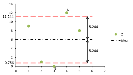
Figure 3: Dataset Z used as an example to explain the standard deviation
The mean ![]() of the dataset Z is 6.0. The standard deviation s = 5.244 gives an estimate of how much the data points are dispersed around the mean line. It indicates that most points lie within a distance of 5.244 above and below the mean line. The boundaries are shown by the red dashed lines in the figure above. Some points (e.g. A and B) may lie outside these limits, but most of them lie, on average, between the limits
of the dataset Z is 6.0. The standard deviation s = 5.244 gives an estimate of how much the data points are dispersed around the mean line. It indicates that most points lie within a distance of 5.244 above and below the mean line. The boundaries are shown by the red dashed lines in the figure above. Some points (e.g. A and B) may lie outside these limits, but most of them lie, on average, between the limits ![]() and
and ![]() .
.
Figure 4 shows a real world example using MajesticSEO’s TrustFlow metric for a particular URL. The number of data points, n = 72, the mean has a value of 9.81. The average squared deviation is calculated to be 60.77 and the variance is 61.62. The standard deviation of the data is equal to the square root of the variance, and has the value 7.85. Thus, most of the points lie within the limits (9.81 – 7.85 = 1.96) and (9.81 + 7.85 = 17.66), as indicated by the red dashed lines in figure 4.
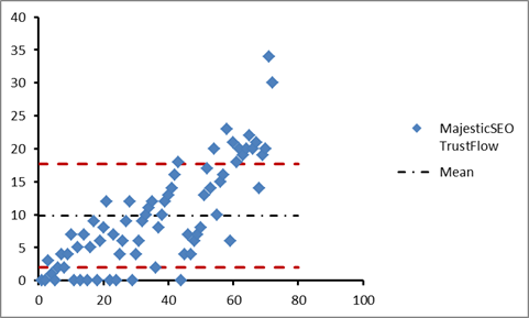
Figure 4: Example using MajesticSEO’s TrustFlow Metric
To recap, we have defined a set of measures that are used for statistical evaluation of a dataset, namely, the mean, average squared deviation, variance and the standard deviation. Then again, all the previous measures of dispersion and central tendency that we have examined so far are solely one-dimensional in nature. Examples of data sets that this type of measure applies to could be: weights of all adults between the ages of 18-24 in the USA, blood pressures of all patients in Hospital A, etc.
However, all data sets are not necessarily one-dimensional; many are multidimensional, and the objective of statistical exploration of these types of data sets is typically to determine the inter-relationship between the dimensions. For example our data may comprise of both the number of hours students in a class spent revising, and the exam scores they received. A statistical analysis could them be carried out to see if the number of hours spent revising has any effect on the grades obtained. The mean and variance only function in one dimension; it is thus possible to calculate only the mean or variance for each dimension of a data set independently of the other dimensions. However, it would be useful to have a similar measure to observe the amount of variability of the dimensions from the mean with respect to each other, which is what correlation is about anyway. We shall expand on these topics in more detail in the next part.
- Ranking of Top Data Scientists on Twitter using MajesticSEO’s Metrics - August 19, 2014
- Measuring Twitter Profile Quality - August 14, 2014
- PageRank, TrustFlow and the Search Universe - July 7, 2014
its too complicated and also in math language which is very difficult for me ………
June 26, 2013 at 7:30 pm> Hi:
I would read parts 1 and 2 for a non-mathematical reference to correlation.
June 27, 2013 at 3:49 pmTerrific maths recap Neep!
I think your end-of-post-3 link to post-4 is missing, or maybe just my groaning browser not showing it?
If its not just me, for everyone else, here’s part 4
July 18, 2013 at 8:56 amhttp://blog.majesticseo.com/research/majesticseo-beginners-guide-to-correlation-part-4/
I’ll fix that now.
July 18, 2013 at 11:49 amDear Neep,
thank you very much for your tutorial. I have never thought, that I will need again my mathematics I learned in school. After school I went to study fine arts, but with the erasing of the new economy I get involved in the WWW, doing SEO since round about 15 years.
I now understand better the Link fight profile charts from MajesticSeo.
What I am asking me, how I can do myself these correlation charts in Excel or some other program from data provided by Google WMT, MajesticSeo, OSE, Sistrix and Linkresearchtools among others, because every data provider shows a own point of view taking from different samples of the same population: domains.
I am think about to translate to German your four parts for my own website http://www.suchmaschinen-experte.de about SEO given you and MajesticSeo the credits.
This would be okay?
Greetings from Hamburg, Germany.
July 18, 2013 at 9:50 amThat would be fine I think.
July 18, 2013 at 11:49 am> Thanks, i will inform you, when it is online.
July 18, 2013 at 1:59 pmHi Hans:
There are many ways to produce correlation charts in Excel. I have provided two links below:
How to calculate Correlation Coefficients in Excel-2010
correlation-matrix-using-excel.htm
July 18, 2013 at 12:15 pm> Sorry about that:
The second link should be:
Correlation Matrix Using Excel
Neep
July 18, 2013 at 12:24 pm>Yet another attempt. Browser is acting up.
July 18, 2013 at 12:30 pmCorrelation Matrix Using Excel
> Thanks, i will check your links. Hans
July 18, 2013 at 2:00 pm> Sorry Neep, again me, i cannot open your second link. I am bookmarking me these links to do later a research. Thanks for your time, Hans
July 18, 2013 at 2:06 pm> Reposting second link again. Browser is acting up.
Correlation Matrix Using Excel
July 18, 2013 at 2:25 pm> HI Hans:
Sorry again. Here is the text version of the link
http://www.listendata.com/2013/02/correlation-matrix-using-excel.html
Also, look up Google for correlation matrix excel
Neep
July 18, 2013 at 5:30 pm